Data Products
NIPS has several different data products dependent on the pipeline step and mode. The list of all products and their documentation can be found here. In the following sections the usage and retrieval of those products will be explained in detail.
Data Retrieval
There are several ways of retrieving nips data products 1) directly from a pipeline run, 2) using one of the pipeline load methods within the pipeline framework (but without having to run the full pipeline again) or 3) using the standalone data product modules.
1) Retrieving data from a pipeline run
If one wishes to obtain the current processed data from the pipeline one can access it through:
# Obtaining the processed data
###############################
data = pl.datainput['S200A1']
This returns an instance of the I2D, R2D, R1D, I1D or R3D class, dependent on which pipeline step was run last. Note, that the slitid is always needed to obtain the right data as the pipeline stores the data of different targets in a dictionary.
> print(pl.datainput)
> {'S200A1': <nips.products.irr2d_module.I2D at 0x181ac817b8>,
   'S200A2': <nips.products.irr2d_module.I2D at 0x181ad1c3c8>,
   'S400A1': <nips.products.irr2d_module.I2D at 0x181ac81128>,
   'S1600A1': <nips.products.irr2d_module.I2D at 0x181acad3c8>,
   'S200B1': <nips.products.irr2d_module.I2D at 0x181ae33dd8>}
2) Retrieving data without re-running the pipeline
If it is desired, one can set up the pipeline environment without rerunning the pipeline as already described in NIPS usage:
# Construct pipeline parameters object
######################################
pl_parameters = PipelineParameters()
pl_parameters.m_set(output_path, archive_path, ref_path, mode,
                    set_from_file=True)
    # Initialize the pipeline class
###############################
pl = Pipeline()
pl.m_set(pl_parameters)
Warning
This is still under development and might not work perfectly yet.
With this in hand, one can now take advantage of the pipeline internal load function (m_load_input()) that handle paths and data retrieval:
    # Load a pipeline product into the pipeline instance
####################################################
pl.m_load_input('AWCS','I2D')
This will load the AWCS products (which is a 2D unrectified spectrum) into the pipeline instance and can be accessed with the pl.datainput attribute as described in 1) Retrieving data from a pipeline run.:
# Obtaining the processed data
###############################
data = pl.datainput['S200A1']
Note
The disadvantage of this method is, that the archive path and reference path have to be set and accessable, even tho they are not used.
3) Retrieving data with standalone modules
The third and post straight forward option would be to use the internal nips data modules directly to load nips products. The advantage: one does not have to set up the entire pipeline environment (including having a archive connected to your computer), the disadvantage: one needs to know the exact path to the products which might be cumbersome considering the complex nips output folder structure.
All datamodules can be access from the pipeline separately. For example:
# Importing data modules
########################
from nips.products.irr2d_module import I2D
from nips.products.reg1d_module import R1D
All modules have a read method (e.g. I2D.m_read_from_fits()) that can be used to load the corresponding data product, for example:
# Initializing and loading
##########################
data = I2D()
data.m_read_from_fits('./master/data/3162_OTIS_OPAQUE_G140H_LINE1/3162_OTIS_FS_S200A1_INTERNAL/products/3162_OTIS_FS_S200A1_INTERNAL_RECT_R2D.fits')
Data Usage
Once the data is loaded, one can perform all operations from that data class and access the data directly:
Accessing the data
For all data classes, the actual data and its extensions are stored in a dictionary:
> print(data.dic_ext.keys())
> dict_keys(['BASE', 'AWCS', 'PAMP', 'WLZP', 'DFLT', 'SFLT', 'FFLT',
  'IFLT', 'PTHL', 'BARS', 'RADM', 'MSBG'])
> print(data.dic_ext['BASE'].keys())
> dict_keys(['data', 'var', 'quality', 'j', 'i', 'header'])
> print(data.dic_ext['BASE']['data'])
> [[array([[-2.05958936, -2.08360142, -4.00976163, ..., -2.77837828,
       0.56195496,  1.8292929 ],
     [ 2.16910314,  1.46586888, -6.06662296, ...,  4.60136928,
       0.96560349,  1.16134612],
     [ 6.12821169,  5.56432763,  4.66260883, ...,  0.63502265,
       4.60629836,  4.36887296],
     ...,
     [-5.41452931, -2.26259031, -0.4216486 , ...,  3.68541563,
       7.0094752 ,  1.73910273],
     [-5.72352554, -0.21688973, -5.47215147, ..., -0.64551099,
       4.01265696,  1.44492133],
     [ 1.49714654,  4.52504853,  2.19282563, ..., -4.9055018 ,
      -1.96947793, -0.27133887]]),
    array([[ 0.18557754,  0.52402179,  4.90271213, ..., -2.0091825 ,
       1.97070749, -0.29821096],
     [-3.6339946 , -5.96464385, -0.818975  , ..., -2.49024459,
       1.09733757, -3.15562565],
     [-6.37640831,  0.962122  ,  3.44608383, ...,  0.56545415,
      -4.32880161, -9.35084114],
     ...,
     [-8.79804632, -5.40014104, -5.94243897, ..., -1.86094089,
      -6.28997709, -6.41994295],
     [ 0.58162118, -2.1468002 , -1.85595475, ..., -3.84111774,
      -4.25929026, -1.47670818],
     [-0.9880203 ,  1.38784672, -3.13343194, ...,  5.63168467,
      -7.65517873, -1.59880356]])],
    'DATA',
    'data',
    None,
    'data array list']
From this is becomes clear that to obtain the actual trace from the twp sca one would do:
# Trace on 491 and 492
######################
trace_491 = data.dic_ext['BASE']['data'][0][0]
trace_492 = data.dic_ext['BASE']['data'][0][1]
and for the wavelength:
# Wavelength on 491 and 492
###########################
lambda_491 = data.dic_ext['AWCS']['w'][0][0]
lambda_492 = data.dic_ext['AWCS']['w'][0][1]
arguments.
For regular products such as R1D, R2D, and R3D the wavelength information is not stored in an extra array but in the wcs of the class. In the R1D, the R1D.m_get_wavelength() can produce a wavelength array from the wcs keywords:
# Wavelength array from R1D object
##################################
lambda_arr = data.m_get_wavelength()
More examples on how to use the different data classes can be found in the description of each data class here.
Saving the data
The m_write_to_fits methods (e.g. I2D.m_write_to_fits()) that are present in all data modules make it easy to save the data product at a custom location:
# Saving output data
####################
data.m_write_to_fits('./output/my_irr2d_data.fits')
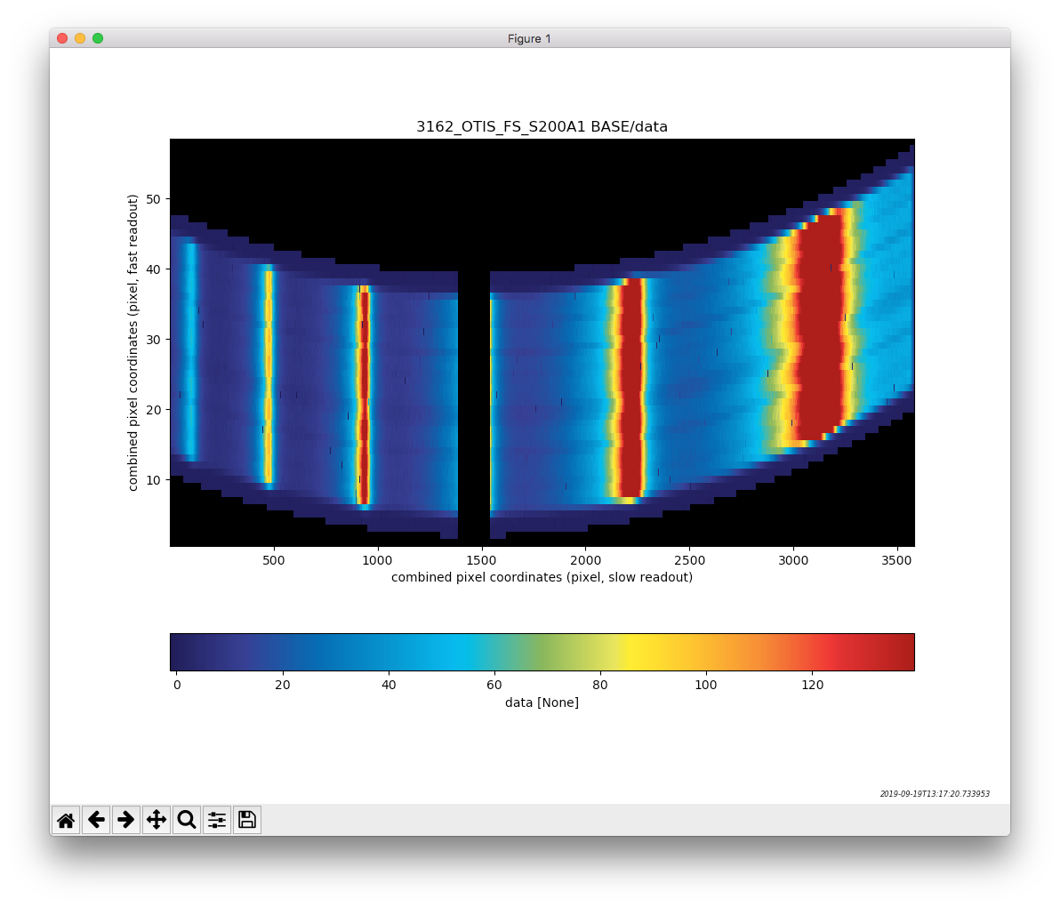
Visualizing the data
Another function that comes with the data products is to display the data. This is done with the m_display method (e.g. I2D.m_display())
# Displaying the data
#####################
fig = data.m_display(close=False)
# Saving the displayed data to file
###################################
data.m_display(filename='./output/my_irr2d_data.pdf')