Pipeline Steps (nips.modules)

As described here, the pipeline is build-up by individual modules of pipeline steps. Each of those step modules is constructed in the same way:

1. Parameters Class:

   Handles all user-given and default parameters for this step.

2. Configuration Class:

   Handles the reference files, performes checks and prepares all additional inputs for the us in the step.

3. Step Class:

   Performes the actual pipeline step.

In addition to those three classes, a step in general also needs the associated reference file class to read and pass the reference file. To run an individual step, the user would have to initiate the parameters, configuration, and step classes as well as the reference file and data classes. The following example illustrates this for the DLFT step:

# ===== DATA INPUT =====
# Filename for data input file - in pipeline we don't need this as we use the output of previous step
datainput = I2D()
datainput.m_read_from_fits(filename_input)

# ===== REFERENCE FILES =====
# Filename for reference file - in pipeline this will be generated by f_find_ref_files
dfltref = DfltRef()
dfltref.m_read_from_fits(filename_ref)

# ===== PARAMETERS =====
dfltpar = DfltParameters()
dfltpar.m_set_default()

# ===== CONFIG =====
# The config class
dfltconfig = DfltConfig()
dfltconfig.m_set(dfltref, dfltpar, datainput)

# ===== STEP =====
# The step class
dfltstep = DfltStep()
dfltstep.m_set(dfltconfig)
# Here we are doing the actual pipeline step
dfltstep.m_step()
# Here we apply it to the data
dfltstep.m_apply()
dfltstep.m_output()

# ===== OUTPUT =====
# The dflt specific data output class
dfltstep.dataoutput.m_write_to_fits('outputfile_dflt.fits')

An alternative to this process would be using the Step class, which is used by the pipeline to perform those steps in an automated way.

In the following sections the pipelien steps will be described in detail.

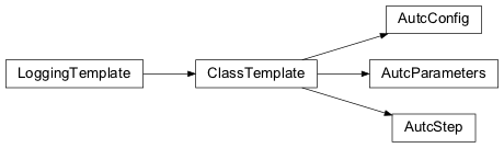
Autocal Correction (AUTC)

The Autocal-correction step divides the data by a lamp observation (taken with the same GWA position) on count-rate level before processing it further for the purpose of flat-fielding. If this step is performed, no further flat-fielding (DFLT, SFLT, FFLT) is needed.

Warning

This module is not complete yet. It is currently only dividing the two exposures and does not take the lamp spectrum into account. This will be changed in the future.

nips.modules.autc_module Module

Classes

AutcParameters([logger_id])	Class for the computation parameters of the Autocal correction step.
AutcConfig([logger_id])	Configuration class for the Autocal correction step.
AutcStep([logger_id])	Step class for the AUTC step.

Class Inheritance Diagram

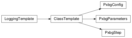
Pixel Background Correction (PXBG)

The pixel background correction divides the data by a background observation on count-rate level before processing it further. This can only be done with observations that were done with the same GWA position.

nips.modules.pxbg_module Module

Classes

PxbgParameters([logger_id])	Class for the computation parameters of the pixel-level background subtraction step.
PxbgConfig([logger_id])	Configuration class for the pixel-level background subtraction step.
PxbgStep([logger_id])	Step class for the PXBG step.

Class Inheritance Diagram

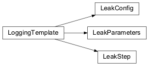
Leakage Correction (LEAK)

The Micro-Shutter Assembly (MSA) of the JWST/NIRSpec instrument is mounted at the FORE optics focal plane and consists of a 2x2 mosaic of quadrants each containing 62 415 micro shutters. This results in ∼ 250 000 shutters in total, each equipped with a shutter door that can be opened and closed using a combination of mag- netic arm moves and individually controlled voltages to ”latch” the shutter. Ideally, when a shutter is closed, light behind that shutter should be blocked, leaving the detector to receive light only from those shutters with open doors. However, this is not entirely the case in reality.

There are two primary effects of leakage:

1. Failed open shutters (FO) - shutters that are permanently open or the doors being stuck open or dam- aged.

2. MSA print-through - a regular pattern that is common to all shutters with slight variations in contrast.

The contrast of failed open shutters vs. leaked light through closed shutters is about 0.004%.This small con- tribution is enhanced in dispersed mode when about 700 shutters pile up in spectral direction, enhancing the contribution of light leaking through the shutters up to almost 3%. This will impact observation of faint sources in bright background environments with the integral field unit (IFU), as the IFU and MSA traces share the same detector space. The only way around it is to take a so called leakage exposure - an exposure with the IFU closed and the MSA closed, ideally with the same exposure time as the science exposure in order to subtract those two from each other on count-rate level. The Leakage Correction subtracts the leakage exposure from the science exposure on count-rate level.

Warning

This module is not implemented yet.

For more information see ESA-JWST-SCI-NRS-TN-2017-051.

nips.modules.leak_module Module

Classes

LeakParameters([logger_id])	Class for the computation parameters of the MSA-leakage subtraction step.
LeakConfig([logger_id])	Configuration class for the MSA-leakage subtraction step.
LeakStep([logger_id])	Step class for the LEAK step.

Class Inheritance Diagram

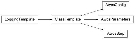
Assign WCS (AWCS)

This is the class for the spectrum extraction and WCS assignment step of the NIPS pipeline.

nips.modules.awcs_module Module

Classes

AwcsParameters([logger_id])	Class for the computation parameters of the extraction and WCS assignment step.
AwcsConfig([logger_id])	Configuration class for the extraction and WCS assignment step.
AwcsStep([logger_id])	Step class for the AWCS step.

Class Inheritance Diagram

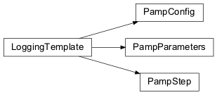
Pixel Area Map Computation (PAMP)

As part of the absolute radiometric calibration for extended sources (i.e. to get a surface brightness), it is necessary to divide the measured spectrum by the surface on the sky covered by a given pixel (for slit-type spectroscopy this is the projected width of the aperture multiplied by the project size of a pixel along the spatial direction).

Due to optical distortion, this value can change as a function of position within the field of view and instrument configuration.

Note that the contribution of variations of the aperture width and the spectrograph to the pixel area map is included in the internal flat-field correction so we only have to worry about the contribution of the optical elements upstream from the MSA (OTE & FORE).

Currently, the PAMP correction is a single number applied to all pixel. For consistency, and potential future improvement (addition of wavelength variation), this method creates a 2D correction array with a value for each pixel.

nips.modules.pamp_module Module

Classes

PampParameters([logger_id])	Class for the computation parameters of the extraction and WCS assignment step.
PampConfig([logger_id])	Configuration class for the Pixel Area Map correction.
PampStep([logger_id])	Step class for the Pixel Area Map correction.

Class Inheritance Diagram

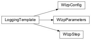
Wavelength Zero Point Correction (WLZP)

NIRSpec operates mostly in diffraction-limited regime and over a large wavelength range (almost a decade in wavelength). As a consequence, the size of the point-spread function (PSF) varies a lot and it was not possible to select aperture sizes that would match the width of the PSF at all wavelengths. In addition, NIRSpec was optimised for observations of faint objects so the choice was made to use slightly oversized apertures with a typical width of 200 milli-arcseconds for the micro-shutters and the standard slits. As a consequence strong intensity gradients can be present across the aperture and NIRSpec is susceptible to the so-called “slit-effect” where an imprint of the intensity distribution of the object across the slit will be present in the spectral PSF.

To first order, this means that for compact sources and in particular point sources the position of the barycentre of the spectral PSF will depend on the centring of the source in the aperture. It will also be different from the one measured in the uniform illumination case, i.e. from the one used for the wavelength calibration of NIRSpec. A wavelength offset of a fraction of a pixel will therefore be present that needs to be corrected.

The main parameters are the wavelength, the aperture itself and the centring of the point source across the aperture.

The correction will be computed when preparing the 2D irregular data product. This data product will contain for each of its pixel: the wavelength lambda_pixel (assumed to be in meter); the dispersion eta_pixel (assumed to be in meter per pixel). On input, we also need the position of the point source within the aperture dx along the spectral direction (expressed in fraction of the aperture width [for slits] or pitch [for micro-shutters]; zero corresponding to a centred source). For each pixel the wavelength correction will be computed as:

\[\delta\lambda_{\text{pixel}} = \eta_{\text{pixel}} x \Delta_{\text{interpolated}}(\lambda_{\text{pixel}}, \delta x_{\text{source}})\]

In this equation, \(\Delta_{\text{interpolated}}\) is the linear interpolation of the reference file data at \((\lambda_{\text{pixel}}, \delta x_{\text{source}})\). No extrapolation should be performed (correction value set to zero and a quality flag tracking the absence of correction should be set).

For more information see ESA-JWST–SCI-NRS-TN-2016-018.

nips.modules.wlzp_module Module

Classes

WlzpParameters([logger_id])	Class for the computation parameters of the extraction and WCS assignment step.
WlzpConfig([logger_id])	Configuration class for the wavelength zero-point correction
WlzpStep([logger_id])	Step class for the wavelength zero point correction.

Class Inheritance Diagram

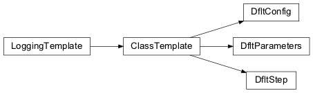
Detector Flat Correction (DFLT)

The conversion from photons to electrons, and ultimately to electronic counts or Data Numbers (DN) is determined solely by the properties of the NIRSpec detector system, i.e. the two Sensor Chip Assemblies (SCAs) with their respective ASIC. At a given wavelength, each of the 2048x2048 pixels of a given SCA has a slightly different Quantum Efficiency (QE). In addition, the QE fluctuations also vary with wavelength, and these variations must be captured across the entire detector.

The spatial uniformity of the flat-field response of the NIRSpec detectors has been measured at 39 wavelengths spanning the entire NIRSpec wavelength range of 0.7 − 5.3μm. These exposures, which were obtained at subsystem level (i.e. before integration into NIRSpec) illuminate the SCAs uniformly and with monochromatic light. In addition, the behavior of the anti-reflection coating has been measured at high spectral resolution by the vendor (Teledyne Imaging Systems). Both data sets are used to create a detector flat-field reference file (D-Flat) which allows to correct for the QE of any pixel at the wavelength(s) of the incoming photons.

The D-flat reference file for each NIRSpec SCA consists of two parts, a data array with 39 QE maps that trace the pixel-to-pixel variations as a (slow) function of wavelength, and a single “fast” vector that captures the fine detail of the AR-coating at 201 wavelengths. This vector is applied equally to all pixels (at their respective wavelength).

The correction value is computed by interpolating the array at the sca coordinates (\(x_{sca}, y_{sca}\)) in wavelength direction times the interpolated value from the vector \(\Delta_{\text{interpolated}}(\lambda_{\text{pixel}})\).

\[\eta_{\text{pixel}} = \text{dflt}_{\text{interpolated}}(\lambda_{\text{pixel}}, x_{sca}, y_{sca}) * \Delta_{\text{interpolated}}(\lambda_{\text{pixel}})\]

For more information see ESA-JWST-SCI-NRS-TN-2016-005 and SA-JWST-SCI-NRS-RP-2016-004.

nips.modules.dflt_module Module

Classes

DfltParameters([logger_id])	Class for the computation parameters of the DFLT correction step.
DfltConfig([logger_id])	Configuration class for the D-flat
DfltStep([logger_id])	Step class for the D-flat

Class Inheritance Diagram

Spectrograph Flat Correction (SFLT)

Most throughput corrections are highly wavelength-dependent. Therefore, flat-fielding of NIRSpec data can only occur after the wavelength falling onto a given pixel has been determined. In other words, the throughput correction of NIRSpec spectra must be computed ”on the fly”, after the spectra have been extracted and specific wavelengths have been assigned to each pixel.

The Spectrograph or S-flat will correct all throughput losses caused between the MSA and the detector. Note that in order to correct the signal in a given detector pixel, the wavelength (range) of light falling onto the pixel must be known. This, in turn, implies that before applying the S-flat correction, the pipeline must first determine which spectral aperture is illuminating the pixel, and must calculate the correct wavelength.

The computation and application of the master S-flat is mode dependent.

FS:

Just like the D-flat, the S-flat is applied on a pixel-by-pixel basis, and each NIRSpec SCA therefore has a ded- icated reference file. Because in fixed slit mode, each detector pixel always receives (almost) the same wave- lengths1, the spatial variations of the throughput can be captured in a single frame (as opposed to a data cube). For each slit, a dedicated vector is needed that captures the behavior of the disperser and the rest of the spectrograph optics at a resolution higher than that of the data, so that a properly sampled throughput vector can be computed at the correct pixel wavelength.

IFS:

Similar to the case of the fixed slits, all NIRSpec IFU exposures illuminate a given NIRSpec pixel with (almost) the same wavelengths. Therefore, a single image extension with the 2048x2048 pixel response map, combined with a single vector is sufficient to flat-field the data.

MOS:

The S-flat reference file in MOS mode contains a (2048 x 2048 x 47) data cube with a 47 wavelength planes, in addition to the finely sampled throughput vector that is identically applied to all pixels. The cube will need to be interpolated to derive the S-flat correction of a given pixel at the correct wavelength.

The correction is computed by looping through each pixel, determining the wavelength lambda_pixel and its pixel position on the sca (\(x_{sca}, y_{sca}\)). For FS and IFS the final correction value is computed by multiplying the s-flat pixel value at (\(x_{sca}, y_{sca}\)) with the interpolated value from the vector \(\Delta_{\text{interpolated}}(\lambda_{\text{pixel}})\).

\[\eta_{\text{pixel}} = \text{sflt}(x_{sca}, y_{sca}) * \Delta_{\text{interpolated}}(\lambda_{\text{pixel}})\]

For the MOS configuration the correction value is computed by interpolating the cube at the sca coordinates (\(x_{sca}, y_{sca}\)) in wavelength direction times the interpolated value from the vector \(\Delta_{\text{interpolated}}(\lambda_{\text{pixel}})\).

\[\eta_{\text{pixel}} = \text{sflt}_{\text{interpolated}}(\lambda_{\text{pixel}}, x_{sca}, y_{sca}) * \Delta_{\text{interpolated}}(\lambda_{\text{pixel}})\]

For more information see ESA-JWST-SCI-NRS-TN-2016-005, ESA-JWST-SCI-NRS-RP-2016-008, ESA-JWST-SCI-NRS-RP-2016-009, and ESA-JWST-SCI-NRS-RP-2016-010.

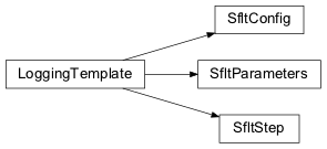
nips.modules.sflt_module Module

Classes

SfltParameters([logger_id])	Class for the computation parameters of the extraction and WCS assignment step.
SfltConfig([logger_id])	Configureation class for the S-flat
SfltStep([logger_id])	Step class for the S-flat

Class Inheritance Diagram

FORE Flat Correction (FFLT)

Most throughput corrections are wavelength-dependent. Therefore, flat-fielding of NIRSpec data can only occur after the wavelength falling onto a given pixel has been determined. In other words, the throughput correction of NIRSpec spectra must be computed ”on the fly”, after the spectra have been extracted and specific wavelengths have been assigned to each pixel.

The FORE+OTE or F-flat will correct all throughput losses caused between the MSA and the and the sky. Note that in order to correct the signal in a given detector pixel, the wavelength (range) of light falling onto the pixel must be known. This, in turn, implies that before applying the F-flat correction, the pipeline must first determine which spectral aperture is illuminating the pixel, and must calculate the correct wavelength.

Just like the D-flat and S-flat, the F-flat is applied on a pixel-by-pixel basis, but what is particular about the F-flat is that it is aperture dependent. Each mode has a dedicated reference file, and additionally, for the FS each slit is treated separatly. For MOS, each quadrant is treated separately.

FS:

NEEDS TEXT

IFS:

NEEDS TEXT

MOS:

NEEDS TEXT

The correction is computed by looping through each pixel, determining the wavelength lambda_pixel and its pixel position on the sca (\(x_{sca}, y_{sca}\)). For FS and IFS the final correction value is computed by multiplying the s-flat pixel value at (\(x_{sca}, y_{sca}\)) with the interpolated value from the vector \(\Delta_{\text{interpolated}}(\lambda_{\text{pixel}})\).

\[\eta_{\text{pixel}} = \text{fflt}(x_{sca}, y_{sca}) * \Delta_{\text{interpolated}}(\lambda_{\text{pixel}})\]

For each quadrant of the MOS configuration the correction value is computed by interpolating the cube at the sca coordinates (\(x_{sca}, y_{sca}\)) in wavelength direction times the interpolated value from the vector \(\Delta_{\text{interpolated}}(\lambda_{\text{pixel}})\).

\[\eta_{\text{pixel}} = \text{fflt}_{\text{interpolated}}(\lambda_{\text{pixel}}, x_{sca}, y_{sca}) * \Delta_{\text{interpolated}}(\lambda_{\text{pixel}})\]

For more information see section 5.5 of ESA-JWST-SCI-NRS-TN-2019_003

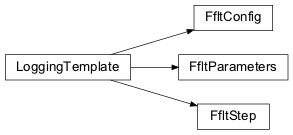
nips.modules.fflt_module Module

Classes

FfltParameters([logger_id])	Class for the computation parameters of the extraction and WCS assignment step.
FfltConfig([logger_id])	Configuration class for the F-flat
FfltStep([logger_id])	Step class for the F-flat TODO: needs update for F-flat, documentation refers to Sflat.

Class Inheritance Diagram

Imaging Flat Correction (IFLT)

The imagging flat is applied to the I2D data by dividing on pixel level.

nips.modules.iflt_module Module

Classes

IfltParameters([logger_id])	Class for the computation parameters of the extraction and WCS assignment step.
IfltConfig([logger_id])	Configuration class for the I-flat
IfltStep([logger_id])	Step class for the I-flat

Class Inheritance Diagram

Pathloss Correction (PTHL)

Aperture losses of light going through the NIRSpec spectrograph are caused mainly by geometric and diffraction losses. Additionally, for uniform-type sources observed through microshutters, although the geometric losses are not relevant, the presence of the so-called microshutter ‘bars’ (the micro-shutters have a filling factor of 63%) will also result in flux losses. Geometric losses (also known as slit losses), occur when the reduced size of the aperture truncates the target. In NIRSpec, as one goes to longer wavelengths, geometric losses increase as a result of the broadening of the PSF due to diffraction. The other contributor to path losses are diffraction losses. The truncation that takes place in the image plane (fixed-slit and micro-shutter apertures, or slicer for the IFU) causes a widening of the illumination that will reach the pupil plane, in this case, the plane of the disperser (or mirror) on the grating wheel assembly, resulting in a partial loss of light.

The pathloss correction uses different reference data for a point source and a uniform illumination.

For both corrections, this method takes the 1D array and interpolates the pthl value for every pixel (given the wavelength at that pixel) and writes it into new pthl correction arrays (one each for point and uniform).

Note that no extrapolations are performed. Wavelength (or source position) values beyond the reference arrays will result in a pthl correction of zero, and a quality flag will track this eventuality.

For more information see ESA-JWST-SCI-NRS-TN-2016-017.

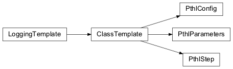
nips.modules.pthl_module Module

Classes

PthlParameters([logger_id])	Class for the computation parameters of the extraction and WCS assignment step.
PthlConfig([logger_id])	Configuration class for the pathloss correction.
PthlStep([logger_id])	Step class for the pathloss correction.

Class Inheritance Diagram

Bar Shadow Correction (BARS)

The micro-shutter “mini-slits” used in NIRSpec MOS mode are not continuous due to the presence of bars between the shutters (micro-shutter aperture height of ~175 microns for a pitch of ~202 microns). These bars will mask part of the sources and backgrounds and this need to be taken into account.

The attenuation for a uniform source is controlled by the profile along the spatial direction of the optical image of the bars on the detectors, any cross talk between neighbouring pixels and the actual sampling of the image of the bar by a given pixel. The shape of the optical image of the bars is a function of:

• The width of the micro-shutter bars along the spatial direction. It is assumed to be identical for all micro-shutters and its value is given by the difference between the pitch and aperture size.

• The point-spread function (PSF) of the spectrograph. The PSF varies with wavelength and with the path through the spectrograph. We have assumed that the dominant effect is the dependence with wavelength and we neglect the variations across the spectrograph (both in terms of position and spectral configuration).

The cross talk between pixels (inter-pixel cross talk = IPC) is assumed to be the same for all pixels.

For more information see ESA-JWST-SCI-NRS-TN-2016-001.

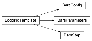
nips.modules.bars_module Module

Classes

BarsParameters([logger_id])	Class for the computation parameters of the extraction and WCS assignment step.
BarsConfig([logger_id])	Configuration class for the bar shadow correction.
BarsStep([logger_id])	Step class for the bar shadow correction.

Class Inheritance Diagram

Radiometric Correction (RADM)

Besides the flat-field correction and the pathloss correction, a final, wavelength-dependent radiometric calibration step for each spectral configuration of each mode is meant to include any residual correction not anticipated and not captured by the other steps.From this point of view, the radiometric correction vector can be seen as a final fudge factor allowing us to cover unanticipated effects or residuals.

By design of the correction itself, the radiometric correction vector is a spectrum (correction factor as a function of wavelength), which will depend on:

• The type of aperture, i.e. MOS, IFU or one of the five fixed-slits.

• The instrument spectral configuration (i.e. the combination of filter and disperser)

The correction will be computed when preparing the 2D irregular data product. This data product will contain the wavelength lambda_pixel (assumed to be in meter) for each of its pixel and we assume that it will also contain the information necessary to identify the associated mode and filter/disperser combination (to be able to select the correct reference file). For each pixel the radiometric correction factor will be computed as:

\[\eta_{\text{pixel}} = \Delta_{\text{interpolated}}(\lambda_{\text{pixel}})\]

In this equation, \(\Delta_{\text{interpolated}}(\lambda_{\text{pixel}})\) is the linear interpolation of the radiometric correction vector at \(\lambda_{\text{pixel}}\). No extrapolation should be performed (correction value set to unity and a quality flag tracking the absence of correction should be set).

For more information see ESA-JWST–SCI-NRS-TN-2016-019.

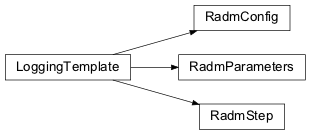
nips.modules.radm_module Module

Classes

RadmParameters([logger_id])	Class for the computation parameters of the extraction and WCS assignment step.
RadmConfig([logger_id])	Configuration class for the radiometric correction.
RadmStep([logger_id])	Step class for the radiometric correction.

Class Inheritance Diagram

Master Background Subtraction (MSBG)

This is the class for the master background subtraction step of the NIPS pipeline.

Warning

This module is not implemented yet.

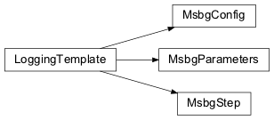
nips.modules.msbg_module Module

Classes

MsbgParameters([logger_id])	Class for the computation parameters of the master background subtraction step.
MsbgConfig([logger_id])	Configuration class for the master background subtraction step.
MsbgStep([logger_id])	Step class for the MSBG step.

Class Inheritance Diagram

Expansion to 2D (EXPD)

This is the class for the R1D -> I2D expansion (for master background) of the NIPS pipeline

nips.modules.expd_module Module

Classes

ExpdParameters([logger_id])	Class for the computation parameters of the extraction and WCS assignment step.
ExpdConfig([logger_id])	Configuration class for the reg1D->irr2D expansion (for master background) step.
ExpdStep([logger_id])	Step class for the EXPD step.

Class Inheritance Diagram

Rectification (RECT)

The rectification module will transform 2D irregular data of the instance of I2D to a 2D regular data instance R2D. This is done by projecting the irregular grid on a regular grid and conserving its flux.

nips.modules.rect_module Module

Classes

RectParameters([logger_id])	Class for the computation parameters of the extraction and WCS assignment step.
RectConfig([logger_id])	Configuration class for the rectification module.
RectStep([logger_id])	Step class for the rectification module.

Class Inheritance Diagram

Rectified Extraction (EXTR)

The extraction module will transform 2D regular data of the instance of R2D to a 1D spectrum data instance R1D. This is done by collapsing the 2D data along the spatial direction, and conserving its flux.

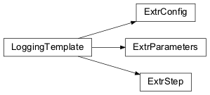
nips.modules.extr_module Module

Classes

ExtrParameters([logger_id])	Class to handle parameters for the 1D extraction.
ExtrConfig([logger_id])	Configuration class for the extraction module.
ExtrStep([logger_id])	Step class for the extraction module.

Class Inheritance Diagram

Irregular Extraction (EXTI)

The extraction module will transform 2D irregular data of the instance of I2D to a 1D spectrum data instance I1D. This is done by collapsing the 2D data along the spatial direction, and conserving its flux.

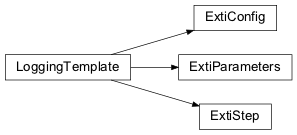
nips.modules.exti_module Module

Classes

ExtiParameters([logger_id])	Class to handle parameters for the 1D irregular extraction.
ExtiConfig([logger_id])	Configuration class for the extraction module.
ExtiStep([logger_id])	Step class for the 1D irregular extraction module.

Class Inheritance Diagram

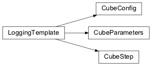
Cube Creation (CUBE)

The cube building module will transform 2D regular data of the instance of R2D to a 3D spectrum data instance R3D. This is done by simply stacking the “slices” into a cube

nips.modules.cube_module Module

Classes

CubeParameters([logger_id])	Class for the computation parameters of the extraction and WCS assignment step.
CubeConfig([logger_id])	Configuration class for the cube building module.
CubeStep([logger_id])	Step class for the cube building module.

Class Inheritance Diagram